
Stronger corporate credit does not automatically produce a stronger equity market. Creditors ask whether promised payments will arrive. Shareholders ask whether the uncertain cash left after those payments justifies the price they pay. A company can become safer for a lender while its shares become less attractive at a higher discount rate.
This article integrates the collection’s original The Asymmetry Has Flipped: An Equity-Flow Case Study, the 1 October report Better credit has not brought the market back, and the 10 September Nifty 50 at the Lower Bollinger Band commentary. The new synthesis separates three questions: solvency, valuation and the timing of marginal demand. Its current evidence was checked on 8 October 2026; observation dates are stated individually.
What the latest verified evidence says
CRISIL Ratings reported 464 upgrades and 213 downgrades in the first half of FY2027, a credit ratio of 2.18 compared with 1.50 in the preceding half-year. Approximately 81% of ratings were reaffirmed. These are observations from CRISIL’s rating universe, not an earnings-growth forecast for a listed index. The release is dated 30 September 2026. CRISIL primary release.
The latest US Treasury daily observation retrieved for this edition is 7 October 2026: two-year par yield 4.77%, five-year 5.03%, ten-year 5.28%, and thirty-year 5.67%. The ten-year figure replaces the source newsletter’s 29 September observation of 5.26% when discussing the current US benchmark. It is a US government par yield, not an Indian corporate borrowing rate or a directly observable equity discount rate. US Treasury daily curve.
These observations support a distinction, not a mechanical market forecast. Better borrower resilience can coexist with a substantial return on relatively safe debt. Whether equities recover also depends on earnings expectations, the equity risk premium, currency effects and participation in the market. The older report’s September oil, rupee, Indian yield, index-return and foreign-flow readings have not been silently advanced to 8 October; this edition does not reproduce them as current quotes.
The financing bridge: base rate plus spread
A useful first approximation is:
Corporate funding rate = matched-maturity base rate + credit spread + fees and other costs.
The source report’s example isolates the mechanism. If the base rate increases by 55 basis points and the credit spread falls by 30 basis points, the simplified borrowing rate still rises by 25 basis points. These changes are illustrative inputs; they are not a statement that every corporate spread moved by that amount.
| Illustrative change | Basis points | Effect |
|---|---|---|
| Base yield | +55 | More expensive benchmark funding |
| Credit spread | -30 | Compensation for credit risk falls |
| Combined simplified funding cost | +25 | Borrowing still becomes dearer |
The transmission depends on the balance sheet. Floating-rate debt reprices according to its benchmark and reset schedule. Fixed-rate debt may defer the cash-interest effect until refinancing. A cash-rich company can earn more on deposits while a highly levered competitor faces a higher funding hurdle. Aggregating these businesses into a single interest-rate sensitivity loses information.
Better credit also does not eliminate a bondholder’s duration loss. A solvent issuer can make every payment while the market price of its fixed-rate debt falls. Default risk, interest-rate risk, liquidity and currency risk need separate entries in a risk register.
A small discount-rate change can matter
For one illustrative payment of Rs100 in ten years, present value is Rs38.55 at a 10.00% annual discount rate and Rs36.68 at 10.55%. The roughly 4.9% decline is arithmetic, not a forecast for an equity index. It uses a single distant payment to make duration visible.
Actual equities contain many possible cash flows. Near-term distributions, reinvestment returns and the uncertainty of growth all matter. A government-yield rise need not pass through one-for-one to the required equity return. If yields rise because real growth improves and earnings rise sufficiently, shares can strengthen. If yields rise because inflation or risk premia increase while margins weaken, the effect can be different.
An earnings yield is therefore a prompt for further work, not an interchangeable alternative to a bond yield. Earnings are not necessarily distributed; a company’s capital requirements can absorb them. A trailing equity CAGR describes a realised historical path, whereas a bond yield is a quotation conditional on contractual cash flows and the assumptions behind that quotation.
A stretched chart is a condition, not a catalyst
The 10 September Nifty commentary used a lower Bollinger Band event to distinguish exhaustion from a persistent trend. The usual construction uses a moving average plus or minus a multiple of a rolling standard deviation. The source’s standard example uses a twenty-day average and two standard deviations. A price outside the lower band can rebound; it can also continue lower as the average and volatility adjust.
The source’s specific claim about four consecutive outside-band closes and a rare September 2022 analogue was supplied as a technical observation, not independently recomputed from a complete price history. It is retained as a historical case premise only. The 23,480 threshold from 10 September is not a live trigger in this edition, and the old “tomorrow” event calendar has been retired.
The reusable decision tree is stronger than the stale level. A close inside the lower band suggests a change in momentum, but still needs earnings, liquidity and breadth confirmation. A rise that remains below the band may be only a bounce within a decline. Another outside-band close suggests persistent pressure, without establishing the next day’s direction. A technical condition alone does not determine position size or provide a calibrated probability of recovery.
Figure 01 · Conceptual framework
Better credit can coexist with a higher borrowing cost
How the parts connect
- Stronger credit qualitypotential spread reliefCredit spread
- Credit spreadcredit componentAll-in funding cost
- Base-rate movementreference-rate componentAll-in funding cost
- All-in funding costfinancing channelEquity valuation
- Base-rate movementdiscount-rate channelEquity valuation
Connect the three horizons
| Horizon | Question | Evidence to keep separate |
|---|---|---|
| Balance-sheet horizon | Can the borrower meet obligations? | Liquidity, leverage, refinancing and ratings |
| Valuation horizon | Do expected shareholder cash flows justify the required return? | Cash-flow forecasts, base rate and equity risk premium |
| Trading horizon | Who is the next buyer or seller? | Breadth, executed flows, positioning and conditional hedge demand |
The original April equity-flow article contributes the third layer. It distinguishes realised past buying from a model of future systematic selling, gross leverage from net exposure, and index performance from constituent breadth. That framework is valuable precisely because it does not allow a favourable observation in one layer to answer every question in the others.
For a more convincing recovery, monitor earnings revisions and margin delivery alongside financing conditions; inspect participation beyond the largest index weights; and distinguish persistent foreign demand from one day’s flow. For a foreign investor, measure the combined local-asset and currency return, including the actual hedge cost if hedged. For a domestic investor, identify imported-input and refinancing exposures inside the portfolio.
No single numerical threshold in the source collection certifies that all three layers have turned. The useful output is a falsifiable decision framework: what would improve the case, what would contradict it, and which facts belong to an earlier date.
Preserved historical analysis
The following April case is retained to preserve the original report’s depth and reasoning. Its positioning numbers, scenarios and market calls remain historical source claims. They are not today’s exposures or executable trading instructions.
The Asymmetry Has Flipped: An Equity-Flow Case Study
A market can retain an upward medium-term bias while becoming vulnerable to a near-term decline. The archived analysis dated 27 April 2026 made precisely that distinction: it preferred convex upside over a one-to-three-month horizon while expecting weaker conditions over the next ten sessions. Its argument rested on the exhaustion of systematic buying, a large pension-rebalancing estimate, compressed hedge-fund exposure and weak breadth at an index high.
This is a historical call reconstruction. The figures and forecasts below belong to that archived analysis and have not been refreshed into current trading instructions. Institutional identities, data-provider names, named securities and author details have been removed. The economic argument is retained, including the weaknesses in its numerical exhibits.
The apparent contradiction at the market high
The source described a broad US equity benchmark as up 9.7% for the month and 4.7% for the year at a fresh high. A price high usually signals that demand has exceeded supply. It does not, by itself, identify who supplied that demand or whether those buyers remain active.
The analysis argued that the market’s marginal buyer had changed. Professional investors had reduced gross exposure, short covering had removed part of a potential future bid, and trend-following systems had largely completed their purchases. It therefore treated the new high as more fragile than the index level suggested.
At the same time, reduced professional exposure could create pressure to participate in a further rise. This was the source of the bullish pain-trade argument. The report did not claim that all investors had become outright short. Its own figures showed substantial positive net exposure. Low gross exposure relative to a recent range is not synonymous with a negative net position.
The source also relied on four selected historical episodes in which the benchmark regained its previous high after a drawdown exceeding 10%.
Source-reported analogue averages
| Comparison | Retained observation |
|---|---|
| One week | It reported average subsequent returns of +1.5% over one week, |
| One month | +5.2% over one month |
| Three months | and +8.6% over three months. |
These were source-reported analogue averages, not forecasts with calibrated probabilities or a complete independent backtest. The small, selected sample supported the original bullish base case but could not establish how the next episode would unfold.
The archived conclusion treated pullbacks as buying opportunities rather than evidence of a market top. That stance coexisted with its tactical downside hedge: the call expected a higher eventual destination while treating the near-term path as hazardous. Recording the analogue figures and the pullback preference preserves the actual historical judgment without endorsing it as a current trade.
Positioning: absolute levels and percentiles
The archived figures distinguished gross and net leverage:
Archived gross and net positioning measures
| Stated measure | Historical value | What it was used to argue |
|---|---|---|
| Fundamental long-short gross leverage | 208.4% | Exposure had compressed relative to its recent distribution |
| Weekly change in gross leverage | −4.6 percentage points | De-risking was continuing into the high |
| Gross leverage percentile | 3rd on a one-year comparison | Positioning was low relative to that sample |
| Net leverage | 51.7% | The sample was still net long |
| Net leverage percentile | 34th | Net positioning was less extreme than gross |
| Monthly reduction in fund shorts | 21.5% | Part of the short-covering demand had already occurred |
Gross exposure adds the absolute size of longs and shorts, while net exposure subtracts shorts from longs. Reducing both sides can lower gross without making the portfolio more bearish. A percentile also depends on the chosen history and sample. Third-percentile positioning over one year is not a statement about every investment manager or every previous market cycle.
The source interpreted the compression as removal of a shock absorber. That is one plausible reading, but the mechanism must be specified. Lower gross can reduce forced-selling vulnerability; it can also indicate that marginal buying demand has faded. Those effects need not point in the same direction. The call relied on the latter effect interacting with the scheduled supply described below.
Systematic buying and conditional future flows
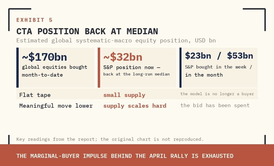
The report estimated roughly $170 billion of global equity buying by trend-following and related systematic investors during the month. It described about $32 billion of long exposure to the large-cap US benchmark, following purchases of $23 billion over the week and $53 billion over the month.
Its central claim was that the systematic community had become a small seller in a flat market and a larger seller if prices fell. That is a conditional model output, not an unconditional forecast of an executed order.
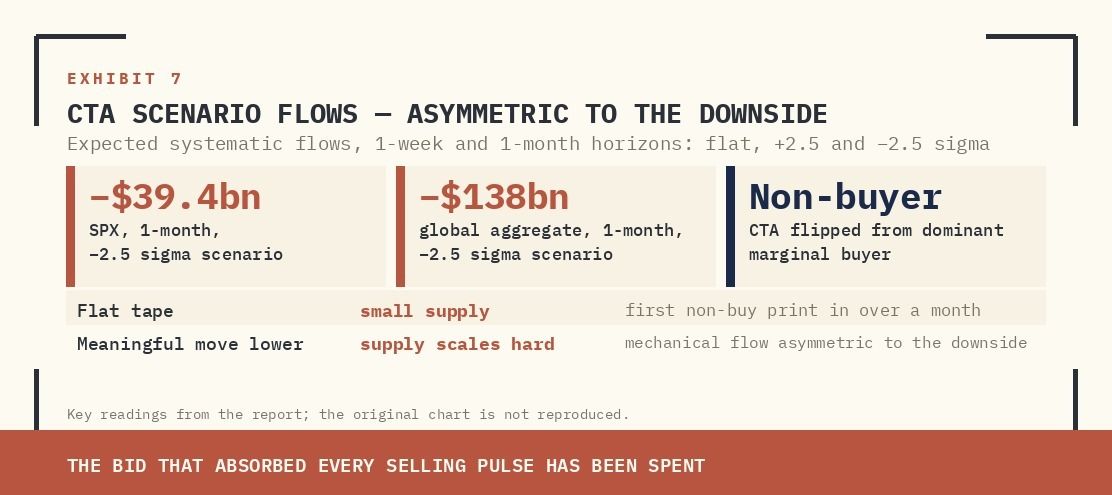
Two downside scenarios were particularly prominent: approximately $39.4 billion of benchmark-related selling over a one-month negative 2.5-standard-deviation move, and approximately $138 billion across global equities under the corresponding aggregate scenario. Neither number should be added to the $170 billion of past purchases as if all three were simultaneous cash flows. They describe different time windows and conditions.
A systematic-flow map is most useful when the assumptions are visible: the trend horizons, volatility targeting, asset coverage and trigger levels. Those model details were not fully recoverable from the narrative. Consequently, the estimates are retained as archived scenario figures rather than independently reconstructed trading-system outputs.
The month-end supply estimate
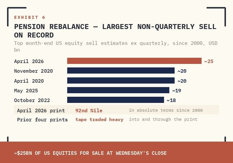
The archived pension-rebalancing estimate was approximately $25 billion of US equity sales. The report compared it with several earlier non-quarterly estimates:
Historical pension-rebalancing comparisons
| Comparison period in the archived table | Estimated selling |
|---|---|
| April 2026 | About $25bn |
| November 2020 | About $20bn |
| April 2020 | About $20bn |
| May 2025 | About $19bn |
| October 2022 | About $18bn |
Pension rebalancing can arise mechanically when equity performance changes portfolio weights. The size of the estimate does not guarantee a matching market impact. Execution may occur over more than one session; other investors may absorb the flow; and the estimate may depend on assumptions about allocation targets and hedging behaviour.
The archived call combined this supply estimate with a concentrated earnings period. It argued that the market would need to digest mechanical sales while a large proportion of index earnings information arrived. The original calendar labels were internally inconsistent, so the operational day-by-day calendar is not reissued here. The economic interaction is preserved without presenting a historical scheduling error as a usable event plan.
Breadth and concentration
Breadth at the archived benchmark high
| Comparison | Retained observation |
|---|---|
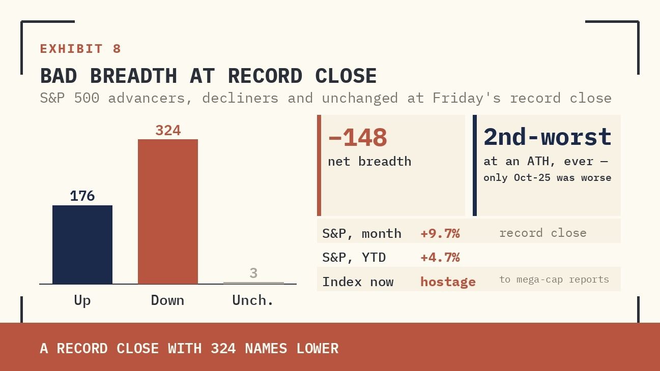
| Advancing | One source exhibit reported 176 advancing names, |
| Declining | 324 declining names |
| Unchanged | and three unchanged names at the benchmark high. |
The arithmetic net advance-decline count was therefore −148. That combination illustrated a market in which a relatively small group of large constituents could lift the capitalisation-weighted index while more constituents fell.
The source also described an eighteen-session winning sequence in a semiconductor benchmark and a large premium to its 200-day moving average. These were used as concentration and extension signals. They do not establish the date of a reversal. A concentrated market can continue rising, especially if the leading companies’ earnings justify their weights.
Breadth matters because it helps distinguish broad participation from dependence on a small set of outcomes. It becomes more informative when combined with valuation, earnings delivery, flows and hedging demand. Treating a single weak-breadth observation as a deterministic sell signal would go beyond the original evidence.
Dealer gamma and the price of convexity
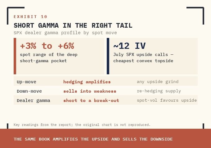
The report argued that dealers were short gamma around a possible breakout. Gamma measures how an option’s delta changes as the underlying price changes. A short-gamma hedge can require buying as the market rises and selling as it falls, potentially reinforcing movement if the hedge flow is large enough relative to liquidity.
The source described a short-gamma pocket over approximately a 3–6% rise and July upside options near 12% implied volatility. Its trade preference was to own convex upside while maintaining downside protection. The appeal depended on the quoted option price, the expected path and the implied-volatility surface, not solely on a view that the index might finish higher.
Option convexity has a cost. Time decay, changes in implied volatility and the timing of the move affect the result. A correct directional view can still produce a losing option trade if the move is too small or arrives too late. The original low-volatility quotation was a historical observation, not a continuously available price.
A numerical inconsistency in the dispersion exhibit
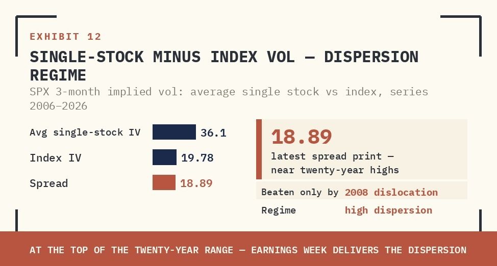
The source reported average single-stock implied volatility of 36.1 and index implied volatility of 19.78, while labelling their spread as 18.89. Simple subtraction gives
The 18.89 figure therefore cannot be reproduced as the direct difference of those two printed inputs. It could reflect a different observation, weighting scheme or tenor, but the archived narrative does not resolve that issue. Both the printed spread and the arithmetic discrepancy are retained rather than silently choosing one.
The broader economic idea is that constituent volatility can differ substantially from index volatility when correlations are low. But a dispersion trade cannot be specified from a simple volatility-point spread alone. Weighting, variance rather than volatility, correlation exposure, option tenor and execution costs all matter.
This is a useful example of preserving a historical thesis while declining to repair its evidence invisibly. The direction of the argument can be intelligible even when an exhibit requires further reconciliation.
The original cross-market positions
The source’s positioning extended beyond the main equity hedge. These calls are recorded as historical views, without named instruments or single-security recommendations.
The original cross-market positions
| Historical position | Source rationale |
|---|---|
| Own convex US equity upside | Low quoted upside volatility and under-participation by professional investors |
| Maintain a tactical equity downside hedge | Rebalancing supply, weak breadth and potential systematic selling |
| Prefer a steeper volatility-index curve | A near-term volatility view differing from the following contract period |
| Own crude downside through a limited-risk option spread | Possible removal of the shipping-disruption premium |
| Prefer selected emerging-market equity exposures | Carry, currency conditions and dispersion |
| Short the euro and sterling | Oil-related terms-of-trade and growth pressure |
| Prefer AI-related power and infrastructure baskets | Capital-expenditure demand and physical bottlenecks |
| Prefer higher-quality consumption over lower-income discretionary exposure | A differentiated consumer and earnings regime |
The currency and commodity calls were conditional parts of a broader portfolio view. They should not be presented as a single hedged package whose risks automatically offset. Different catalysts can arrive at different times, and correlations can change when markets become stressed.
Transmission to India
The archived read-across focused on dollar conditions, foreign portfolio flows, the import bill and industrial investment. A global volatility shock could affect domestic equities through both foreign selling and changes in the currency. Higher oil could pressure the import bill and some downstream margins, while a reduction in the disruption premium could ease that pressure.
The analysis also connected global data-centre investment to domestic power, cooling, electrical equipment and construction demand. This was a sector-level transmission argument. It did not establish that every company exposed to those themes would earn attractive returns or that capital expenditure would arrive on the same schedule.
These channels can diverge. A domestic industrial supplier may benefit from investment demand while facing higher financing costs or imported-input prices. The appropriate unit of analysis is the cash-flow exposure and its valuation, not the thematic label alone.
What the case teaches
The enduring analytical method is to connect positioning, scheduled flows, market breadth and option pricing while keeping their measurement differences visible. Estimates of future selling are not realised flows; low gross exposure is not the same as an outright short position; and an attractive option quotation is not a guaranteed profit. A strong historical report preserves those distinctions as carefully as it preserves its original call.
The original call was explicitly two-speed: a higher forward base case, with near-term vulnerability. It preferred convex participation, downside protection and selective relative-value exposure. No realised outcome has been inserted to make that judgment look better or worse.
Full original report: The Asymmetry Has Flipped
The supplied original is retained below with dated editorial notes. The web analysis above and its corrections remain part of this reading edition.
Original Lens and publication context
Hedge funds have de-grossed into records. The CTA bid is finished. Twenty-five billion dollars of pension supply hits Wednesday’s close. Dealers sit short gamma into the busiest earnings week of the year. The pain trade still points up — but the seatbelt sign is on.
- S&P closed Friday at a record, +9.7% on the month and +4.7% YTD, with the second-worst breadth ever recorded at an all-time high: 176 up, 324 down. The semiconductor index is up eighteen straight sessions, about 50% above its 200-day average.
- The cushion is gone: hedge-fund gross leverage went from the 100th to the 3rd percentile in three weeks (208.4%, net 51.7%), ETF shorts are down 21.5% on the month, and CTAs — buyers of ~$170bn of global equities this month — are done.
- Supply stiffens into the busiest week of 2026: ~$25bn of pension selling at Wednesday's close, the largest non-quarterly sell estimate on record, collides with the most concentrated earnings session ever (~21% of S&P market cap), the Fed, the BOJ and payrolls.
- The surface still pays for upside: July SPX calls trade at a 12 implied vol, dealers are short gamma to a break-out, and a single-stock-versus-index vol spread of 18.89 marks a generational dispersion regime. The forward base case is higher; the path is the trade.
- Position: long convex upside and hedge the supply cliff; VIX curve steepener; long crude downside; long EM equities, Brazil and Korea preferred; short EUR and GBP on Brent 85+; long AI-infrastructure baskets; short low-income discretionary against quality consumer. In India, dispersion favours stock-pickers.
Figure 02 · Qualitative comparison
Three horizons behind an equity recovery claim
| Horizon | Core question | Relevant evidence |
|---|---|---|
| Balance sheet | Can the borrower meet its obligations? | Liquidity, leverage, refinancing and credit ratings |
| Valuation | Do shareholder cash flows justify the price? | Earnings expectations, base yields and equity risk premium |
| Trading | Who is the next buyer or seller? | Market breadth, executed flows, positioning and hedging demand |
EXECUTIVE TAKEAWAY
S&P closed Friday at a fresh all-time high, +9.7% on the month and +4.7% YTD. Underneath the index, the plumbing has rotated 180 degrees in three weeks. Hedge fund gross has gone from the 100th percentile to the 3rd percentile on a one-year lookback. ETF shorts are down 21.5% MoM. The CTA community has bought roughly $170bn of global equities this month and is now done — small seller in a flat tape, meaningful seller on any leg lower. Month-end pension rebalancing prints around $25bn of US equities for sale on Wednesday’s close — the largest non-quarterly sell estimate on record. The index made its high with the second-worst breadth ever recorded at an all-time high.
The cushion has been removed at the same moment the supply schedule stiffens. The pain trade still points up because almost no professional is outright long, July upside trades at a 12 implied vol, and dealers are extremely short gamma to a break-out. But the asymmetry has flipped against the bulls on any tape that goes the other way. Trade the convex upside; size the downside hedge.
TRIGGER
THE SETUP INTO THE GAUNTLET
Busiest week of 2026. Fed and BOJ both decide. 44% of S&P 500 market cap reports earnings; Wednesday alone is the most concentrated single earnings session on record (~21% of S&P market cap), with four mega-caps all post-close. A fifth mega-cap Thursday post-close. Payrolls Friday.
EXHIBIT 1 · EARNINGS CONCENTRATION
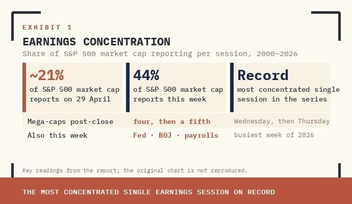
Supplied archive exhibit · original labels. Read alongside the editorial corrections.
The semiconductor index closed Friday up eighteen consecutive sessions — the longest streak ever recorded — and roughly 50% above its 200-day moving average, the largest dislocation since the year-2000 blow-off top. The geopolitical tape has rotated as well: the US–Iran face-to-face track in Pakistan was abandoned over the weekend; the de-escalation premium that drove the last leg of the squeeze now sits exposed to headline reversal. For the first time in weeks, the index trades on actual fundamentals rather than Truth Social tape and Hormuz tickers.
EXHIBIT 2 · SOX OVERBOUGHT SIGNAL
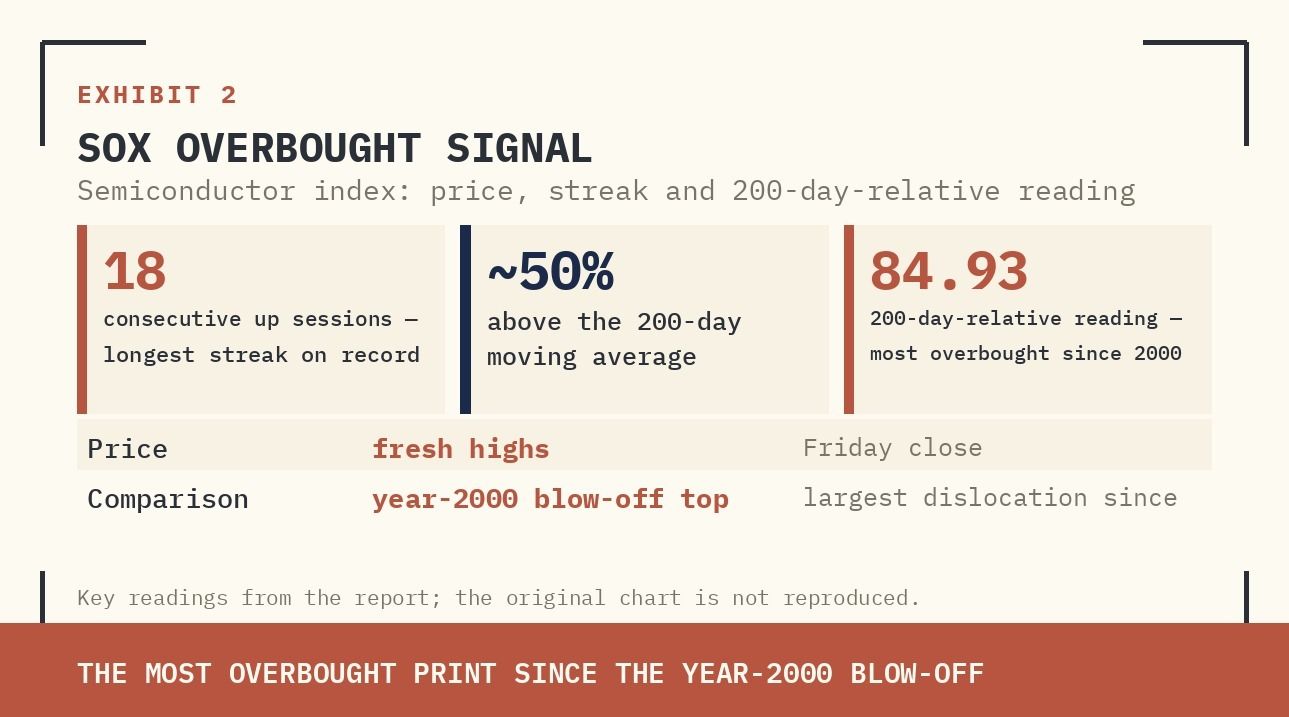
Supplied archive exhibit · original labels. Read alongside the editorial corrections.
FLOW
DE-GROSS, CTA DONE, PENSION CLIFF
Three flow signals matter, and they all point the same way.
One — De-gross. Largest weekly notional de-grossing in seven months. Aggregate gross trading activity declined for the first time in thirteen weeks. US Fundamental L/S gross leverage compressed 4.6pt WoW to 208.4% — 3rd percentile of the one-year range. Net leverage at 51.7%, 34th percentile. The unwind is concentrated in Tech and Discretionary; the prime-book Tech weekly gross-flow Z-score breached −2σ. ETF shorts are down 21.5% MoM. Long-only continued to add Tech into the high; hedge funds were the marginal reducer.
EXHIBIT 3 · RISK EXPOSURES: GROSS AT 3RD %ILE, NET AT 34TH
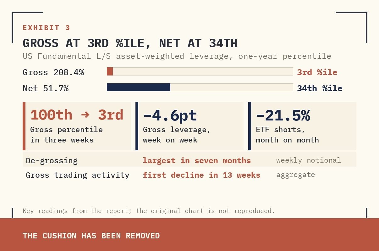
Supplied archive exhibit · original labels. Read alongside the editorial corrections.
EXHIBIT 4 · TECH DE-GROSS AT −2Σ
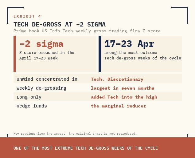
Supplied archive exhibit · original labels. Read alongside the editorial corrections.
Two — CTA done. The CTA community bought ~$170bn of global equities MTD and now sits long ~$32bn S&P after a $23bn week and $53bn month. For the first time in over a month, the model is no longer a buyer. In a flat tape the trigger map shows small supply; on any meaningful move lower, the supply scales hard. The bid that absorbed every selling pulse since the ceasefire has been spent.
EXHIBIT 5 · CTA POSITION BACK AT MEDIAN
Supplied archive exhibit · original labels. Read alongside the editorial corrections.
Three — Pension cliff. April pension rebalance estimate: ~$25bn US equities for sale at Wednesday’s close. Stripping out quarterly expiries, the largest monthly sell estimate ever recorded — 92nd percentile in absolute terms back to 2000. The four prior comparable non-quarterly sell prints each preceded a tape that traded heavy into and through the print.
EXHIBIT 6 · PENSION REBALANCE: LARGEST NON-QUARTERLY SELL ON RECORD
Supplied archive exhibit · original labels. Read alongside the editorial corrections.
TOP NON-QUARTERLY SELL ESTIMATES
ESTIMATE (USD BN) | TAPE BEHAVIOUR AROUND PRINT | |
|---|---|---|
April 2026 (this month) | ~25 | Pending. Bad breadth; HFs 3rd %ile gross; CTA done. |
November 2020 | ~20 | Late post-election rotation; reflation grind. |
April 2020 | ~20 | Post-COVID-low rebalance; deep mechanical supply. |
May 2025 | ~19 | Followed Apr-25 drawdown-and-recapture sequence. |
October 2022 | ~18 | Mid-bear-market low retest; prior episode of forced supply. |
RISK
THE FIVE WARNING LIGHTS
The desk is bracing for a near-term index-level pullback. Five signals are flashing.
SIGNAL | READ |
|---|---|
1. Gross compressed | Hedge fund gross from 100th → 3rd %ile in three weeks. Shock-absorber gone. Net at 34th %ile. |
2. Pension cliff | $25bn US-equity supply at Wednesday’s close — largest non-quarterly sell ever recorded. Collides with most concentrated earnings session in history. |
3. Systematic bid finished | CTA flipped from dominant marginal buyer to non-buyer. SPX 1M −2.5σ scenario prints −$39.4bn; aggregate global −$138bn. Mechanical flow asymmetric to the downside. |
4. Bad breadth at record | Friday: 176 up / 324 down / 3 unchanged; net −148. Second-worst breadth at an ATH ever recorded. Only Oct-25 was worse. Index now hostage to a handful of mega-cap reports. |
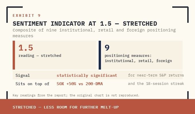
5. Sentiment stretched | Desk sentiment indicator at 1.5 (stretched). Sits on top of SOX 50% above 200-DMA and the longest-ever 18-session streak. |
EXHIBIT 7 · CTA SCENARIO FLOWS: ASYMMETRIC TO THE DOWNSIDE
Supplied archive exhibit · original labels. Read alongside the editorial corrections.
EXHIBIT 8 · BAD BREADTH AT RECORD CLOSE
Supplied archive exhibit · original labels. Read alongside the editorial corrections.
EXHIBIT 9 · SENTIMENT INDICATOR AT 1.5 (STRETCHED)
Supplied archive exhibit · original labels. Read alongside the editorial corrections.
PRICE
Figure 03 · Conceptual framework
Conditional hedging flows can amplify a market move
How the parts connect
- Initial price movedelta changesShort-gamma hedge change
- Short-gamma hedge changeconditional hedge demandPotential amplification
- Available market depthlimits or magnifies impactPotential amplification
- Potential amplificationposition evolvesPositioning reassessment
- Positioning reassessmentrecalculate, do not assume permanenceShort-gamma hedge change
TWELVE-VOL UPSIDE, GENERATIONAL DISPERSION
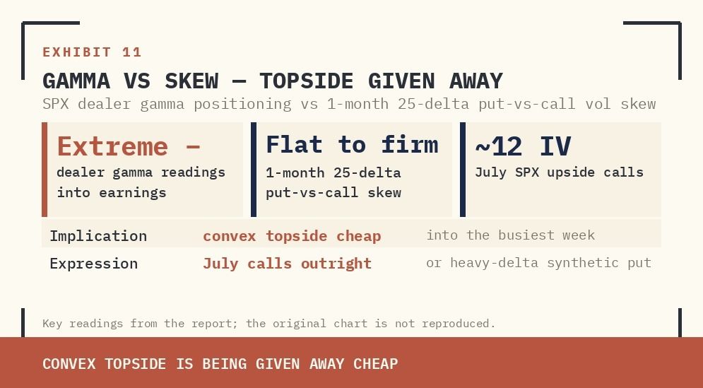
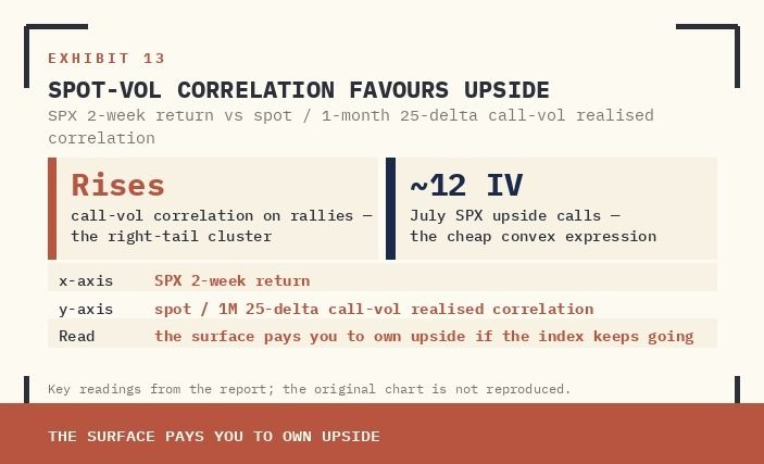
The vol surface tells the positioning story. July SPX upside calls trade with a 12 implied-vol handle — among the cheapest convex bets on the screen. Dealers are structurally short gamma to a break-out, so spot-vol correlation flips in the buyer’s favour on the way up. If the index melts higher into earnings, dealer hedging amplifies the move; if it breaks lower, the same book delivers re-hedging supply that compounds the down-move.
EXHIBIT 10 · SHORT GAMMA IN THE RIGHT TAIL
Supplied archive exhibit · original labels. Read alongside the editorial corrections.
EXHIBIT 11 · GAMMA VS SKEW: TOPSIDE GIVEN AWAY
Supplied archive exhibit · original labels. Read alongside the editorial corrections.
Single-stock-versus-index implied vol sits at generational extremes: average single-stock IV 36.1, index IV 19.78, a simple difference of 16.32 volatility points — at the top of the twenty-year range, beaten in absolute terms only by the 2008 dislocation. The market is pricing a continued low-correlation, high-dispersion regime — exactly the regime in which single-name shorts and pair structures generate the most alpha. Earnings week mechanically delivers the dispersion the surface is pricing.
EXHIBIT 12 · SINGLE-STOCK MINUS INDEX VOL: DISPERSION REGIME
Supplied archive exhibit · original labels. Read alongside the editorial corrections.
The almanac is on the bull’s side over a one- to three-month horizon. In the four post-GFC episodes where the S&P recaptured prior highs after a 10%+ drawdown — Aug-15→Feb-16, Feb-20→Jun-20, Feb-22→Jun-23, and the Apr-25 sequence — forward 1W / 1M / 3M returns averaged +1.5%, +5.2%, +8.6%. The base case is higher. The risk is the path.
EXHIBIT 13 · SPOT-VOL CORRELATION FAVOURS UPSIDE
Supplied archive exhibit · original labels. Read alongside the editorial corrections.
SURFACE READ
READ | IMPLICATION | |
|---|---|---|
July SPX upside calls | ~12 IV | Cheapest convex topside on the screen. |
Dealer gamma profile | Short to break-out | Spot-vol corr favours upside grind. |
Avg single-stock IV | 36.1 | Earnings-week dispersion priced rich. |
Index IV | 19.78 | Generational gap vs single-stock. |
Sentiment indicator | 1.5 (stretched) | Reduces room for further melt-up. |
POSITION
WHERE THE DESK IS LEANING
The trade construction follows the surface and the flow. Long convex upside; short the tail; play the dispersion.
TRADE | STRUCTURE | THESIS |
|---|---|---|
Long SPX upside | July calls outright, or heavy-delta synthetic put | 12-vol topside; lonely positioning; short-gamma dealers. |
VIX curve steepener | Long May VIX puts / short June VIX puts | Front-end pin into earnings, then term-structure rebuild. |
Long crude downside | crude-oil ETF put spreads | Hormuz premium fades on talks-track or supply normalisation. |
Long EM equities | Brazil and Korea preferred | Carry, dispersion, USD path; commodity-currency bid. |
Short EUR / Short GBP | Spot or downside option | Brent 85+ taxes European terms-of-trade and growth. |
Long AI infrastructure | Data-centre and Power-up-America baskets | Capex cycle; token-revenue linkage; constraint pricing. |
Short low-income discretionary | Pair vs quality consumer | Dispersion regime; bifurcated US consumer. |
Tactical SPX hedge | KO puts; lower-spot / lower-yield vol | Cheap protection against pension cliff and breadth break. |
INDIA READ-ACROSS
Four transmission channels matter for the Indian buy side this week.
USD path & FII flows. A US month-end rebalance of this size, layered on stretched sentiment and weak breadth, raises the probability of a vol-up, beta-down impulse exporting through the USD path and SPX–VIX correlation. If it arrives, FII flows turn marginal seller, INR comes under pressure, and Nifty’s mega-cap correlation tightens.
Brent transmission. The desk’s short-EUR / short-GBP is built on Brent 85+. The same crude print is the binding constraint on India’s import bill, OMC marketing margins and CPI trajectory. If oil holds, OMCs stay capped; if the Hormuz premium fades on a talks-track reset, OMC marketing margins reflate fast and the rupee gets a tactical reprieve.
Dispersion plays domestic. The wide single-stock-versus-index volatility gap is the cleanest signal that pair trades and single-name dispersion are pricing alpha. Translation: long quality consumer / short mass-discretionary; long capex-cycle EPC and power transformers / short funded-by-cheap-credit names. The regime favours stock-pickers over directional Nifty exposure.
AI capex basket. The desk’s long AI data-centre infrastructure has clean Indian read-across through the power-and-cooling supply chain — transformers, switchgear, EPC, industrial cables, data-centre REIT-style structures. The token-consumption thesis driving the SOX dislocation transmits into Indian capex names that sell into the same hyperscaler build-out, with a lag and a discount.
ORIGINAL EVENT WATCHLIST — DATE/SESSION MAPPING REQUIRES RECHECK
DAY | EVENT | WHY IT MATTERS |
|---|---|---|
Mon 28 | Tape positioning into Fed week | Watch breadth and HF gross — further compression accelerates Light 1. |
Tue 29 | Macro prints; pre-FOMC vol; ~21% of S&P market cap reports | Most concentrated single earnings session on record. |
Wed 30 | FOMC + four mega-cap earnings post-close + month-end rebalance | Mega-cap earnings collide with $25bn pension supply. |
Thu 01 | Fifth mega-cap earnings post-close; BOJ | Mega-cap close-out; JPY tail risk on policy print. |
Fri 02 | Payrolls; week wrap | First read on whether the pullback was bought or extended. |
BOTTOM LINE
Index at fresh highs on the largest short-squeeze and CTA-buy of the year. Hedge funds de-grossed into the high; CTA bid finished; record-size pension supply hits the most concentrated earnings session ever recorded; breadth among the worst at an ATH; sentiment stretched.
Forward base case higher. Next ten sessions, not. Long convex upside cheap; hedge the supply cliff cheaper; play the dispersion. Treat any pullback as a buying opportunity, not a top.